Correlation - Continuous / Continuous

• Easy
• Pearson correlation coefficient
  • scipy.stats.pearsonr
  $$ r = \frac{\sum_{i=1}^{n} (x_i - \bar{x}) (y_i - \bar{y})}{\sqrt{\sum_{i=1}^{n} (x - \bar{x})^2 \sum (y - \bar{y})^2}} $$
  • Measures linear relationships
  • Symmetric
    : Swapping the two gives the same value
  • Sensitive to outliers
  • homoscedasticity
    • Variance doesn't change

Homoscedasticity vs Heteroscedasticity

Correlation - Pearson's Correlation r

Correlation - Continuous / Ordinal

• Biserial
• Continuous / Ordinal Categorical (dichotomous)
• Kendall's $\tau_{b}$ - rank correlation coefficient
  • Not perfect: meant for ordinal / ordinal
  • scipy.stats.kendalltau
• For large levels (>6) ordinals
  • Pearson correlation coefficient

Correlation - Continuous / Nominal

• Hardest one
• Continuous / dichotomous
  • Point Biserial Correlation
    • scipy.stats.pointbiserialr
    • Far from perfect
    • Assumes Normality
• Continuous / Nominal
  • Correlation Ratio
  • Code
  • Assumes Normality

Adding a variable to the dataset

• Add something that we know is predictive

          df["SeniorCitizenContinuous"] = [
              random.uniform(0.0, 0.5) if v == 0 else random.uniform(0.5, 1.0)
              for v in df["SeniorCitizen"].values
          ]
          

• If SeniorCitizen == 0, random number between (0.0, 0.5)
• else (SeniorCitizen == 1), random number between (0.5, 1.0)

Correlation - Point Biserial

Correlation - Correlation Ratio

Correlation - Ordinal / Ordinal

• Rank ordered categoricals
• Rank Correlation
  • Spearman's rank correlation coefficient
    • scipy.stats.spearmanr
  • Kendall's $\tau_{b}$ - rank correlation coefficient
    • scipy.stats.kendalltau
  • Goodman and Kruskal's gamma
  • Somers' D
    • Untested code

Correlation - Ordinal / Nominal

• Rank-biserial correltion
  • Code (untested)
• For large levels (>6) ordinals
  • Pearson correlation coefficient

Correlation - Nominal / Nominal

• Goodman and Kruskal's lambda
  • Asymmetric
• Cramér's V
  • Symmetric
  • Code
• Tschuprow's T
  • Symmetric
  • Code

Correlation - Cramer's V

Correlation - Tschuprow's V

Correlation - Categorical / Categorical - Which to keep?

• They're correlated, which to keep/remove?
  • Based off response
    • p-value and Z/t-score
      • One variable model
    • Difference with mean of response weighted
      • Higher the better
  • Based off differences
    • Entropy

Entropy

• Information Theory
• Measure of "information" inherent in a variable's possible outcomes
• Best lossless compression
• scipy.stats.entropy

Given a discrete random variable $X$, with possible outcomes $x_{1},...,x_{n}$, which occur with probability $\mathrm {P} (x_{1}),...,\mathrm {P} (x_{n})$, the entropy of $X$ is formally defined as:

$ \mathrm {H} (X)=-\sum _{i=1}^{n}{\mathrm {P} (x_{i})\log \mathrm {P} (x_{i})}$

Principal component analysis

• Dimension reduction technique
  • Continuous variables
• sklearn.decomposition.PCA

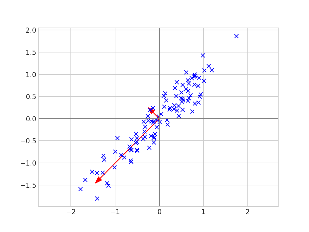
PCA - How does it work

Two Continuous Features

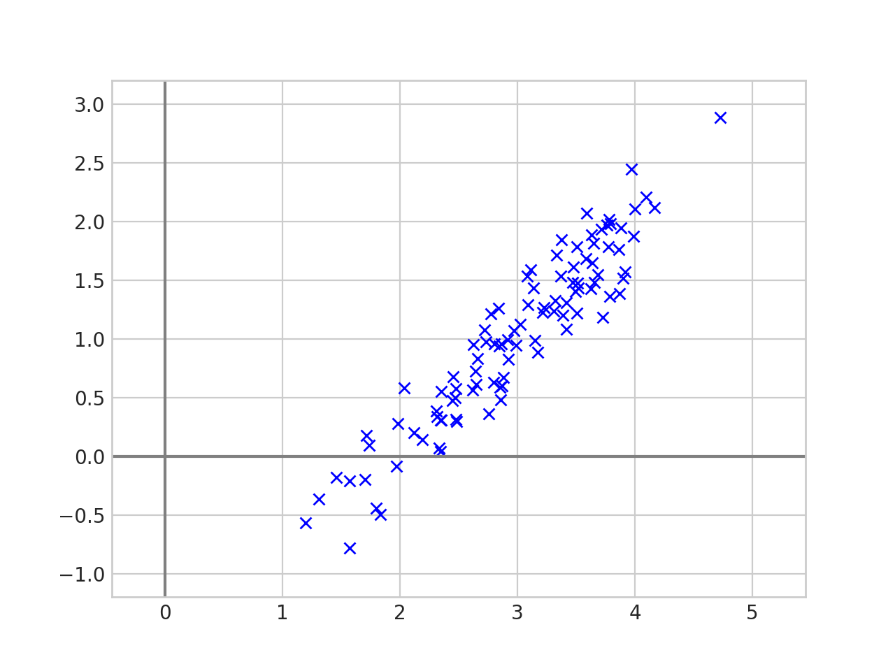
Clear relationship

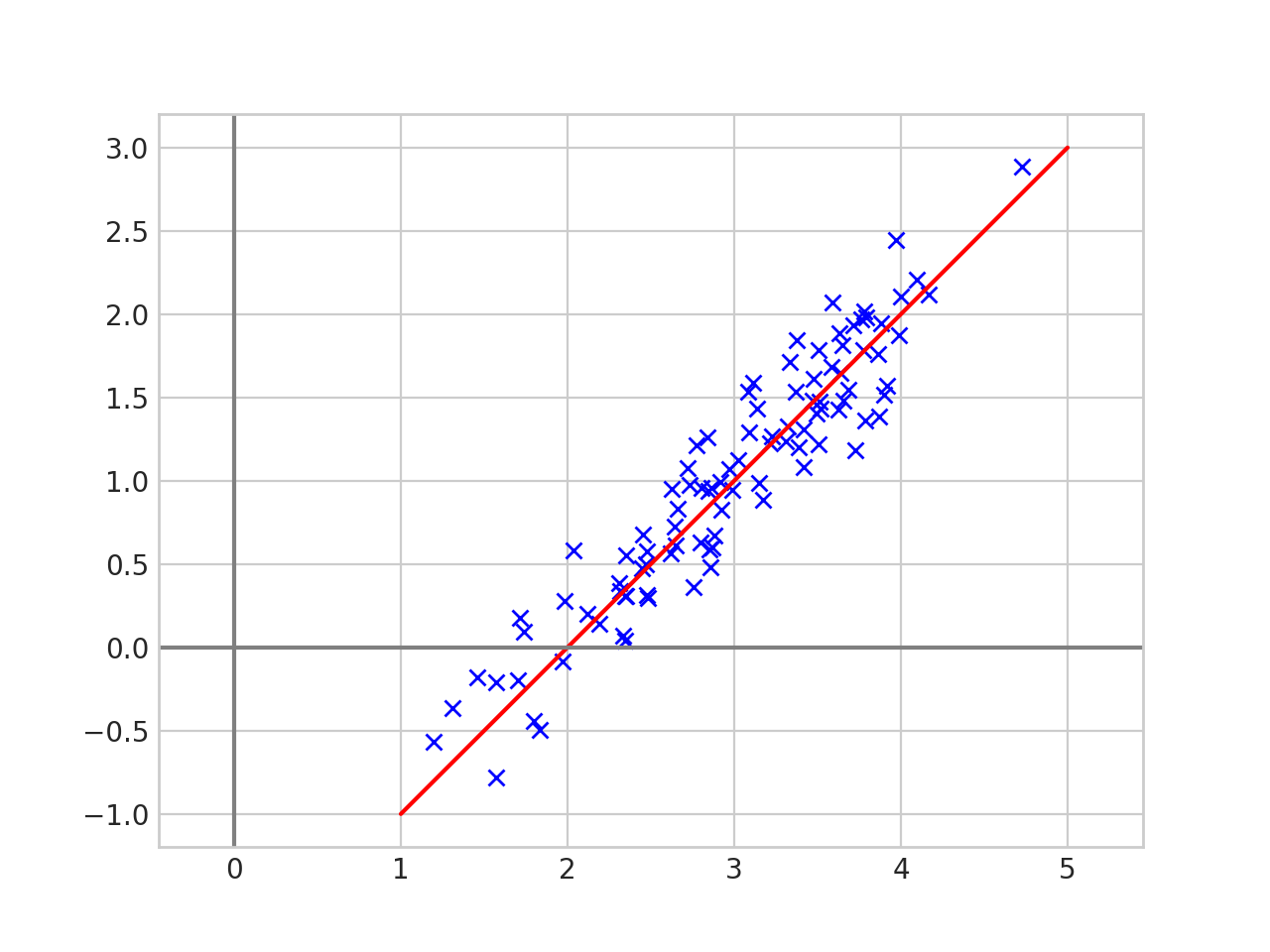
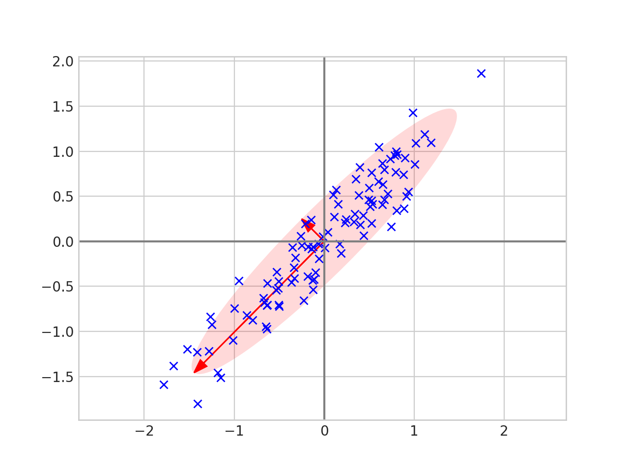
PCA - How does it work

Z-normal

Eigenvectors

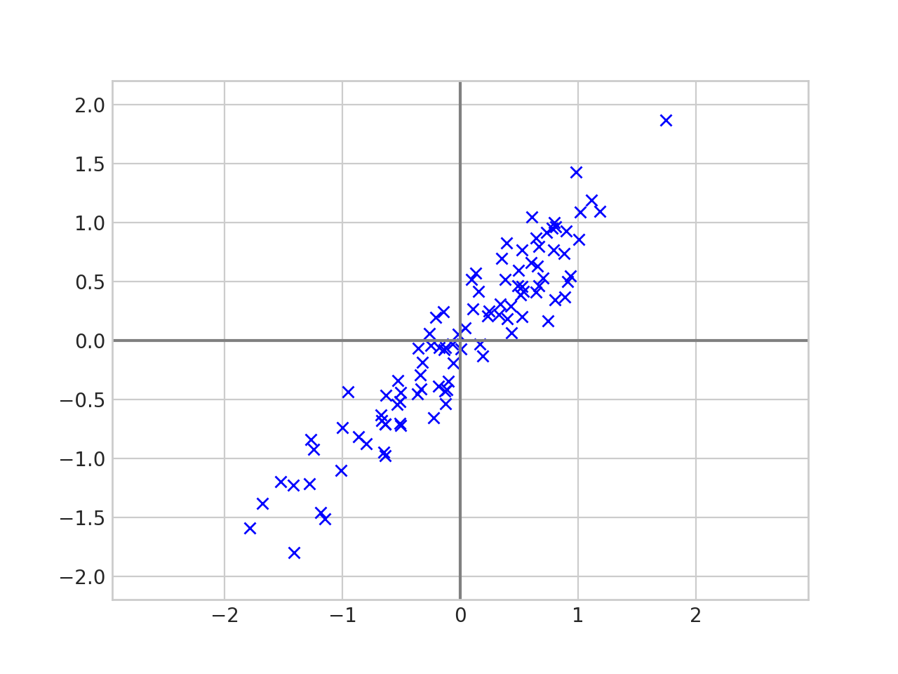
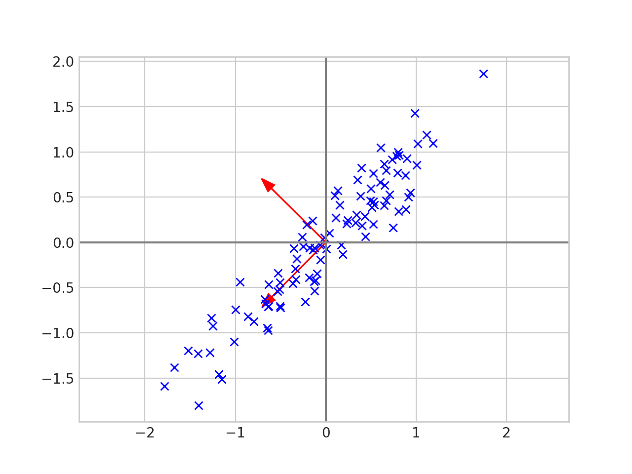
PCA - How does it work

Eigenvalues

Spread

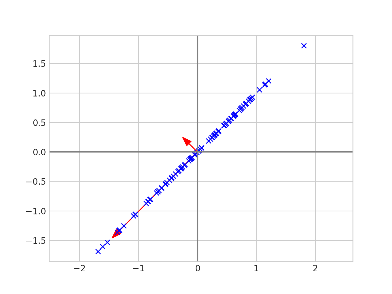
PCA - Collapsed

PCA - Usage

• Usage
  • Don't pick a number of features to use! 😡
  • explained_variance_ratio_
    • Values sum to 1
    • Gives how much of the variance is explained by each component
      • [0.39, 0.32, 0.19, 0.1 , 0. ]
    • Cummulative sum on it
      • [0.39, 0.72, 0.9 , 1. , 1. ]
      • Pick a cut-off, ie: 90% variance explained
• Caveats
  • Lose explainability 📣

Coming Up with New Features

• Imagination!
• Another, combining features together
  • Continuous with continuous
  • Continuous with categorical
  • Categorical with categorical

Continuous with Continuous

• Examples
  • Loan to Value (LTV)
    • Loan / Appraised Value
    • Great indicator of risk
  • Value to Automated Valuation Models (AVM)
    • Appraisal Value / AVM
    • Appraiser commited fraud?
• Coming up with our own
  • Brute force it
    • n=100 variables: $ \binom{100}{2} = 4,950 $
    • n=1000 variables: $ \binom{1000}{2} = 499,500$
    • Get's ugly fast
    • Remove highly correlated variables
      • Lowers the n
      • That wouldn't catch Value to AVM

Continuous with Continuous

• Generate list yourself
• Come up with candidates
  • Plot
    • Check for relationships
    • A heatmap binning both predictors with the value in the bin the difference with the response
    • Operations
      • Divide
      • Plane rotations
• Brute force
  • Hard to do well

Continuous with Continuous - Brute Force

• Ranking
  • Extend the difference with mean of response with an extra dimension
    • Calculate both weighted and unweighted
    • Same as before, just on 2 dimensions
    • The higher the better
• Plotting (2 ways)
  • Plot bin mean $\mu_{(i,j)}$ as the $z$ (height)
    • Must scale the legend so the center is at the population mean
  • Plot like a residual
    • The $z$ (height) in the plot is $\mu_{(i,j)} - \mu_{pop}$ (the bin mean - population rate)
    • Can also plot the weighted version this way

Cont. with Cont. - Difference with mean

No relationship (Bin mean plot)

Cont. with Cont. - Difference with mean

No relationship (Residual plot)

Cont. with Cont. - Difference with mean

No relationship - (Bin mean vs. Residual plot)

Cont. with Cont. - Difference with mean

No relationship (Residual Weighted)

Cont. with Cont. - Difference with mean

No combined relationship (Bin mean plot)

Cont. with Cont. - Difference with mean

No combined relationship (Residual plot)

Cont. with Cont. - Difference with mean

No combined relationship - (Bin mean vs. Residual plot)

Cont. with Cont. - Difference with mean

No combined relationship - (Residual Weighted)

Cont. with Cont. - Difference with mean

Combined relationship - (Bin mean plot)

Cont. with Cont. - Difference with mean

Combined relationship - (Residual plot)

Cont. with Cont. - Difference with mean

Combined relationship - (Bin mean vs. Residual plot)

Cont. with Cont. - Difference with mean

Combined relationship - (Residual Weighted)

Cont. with Cont. - Combined relationship

• They must be correlated! 😏

              x_1 = numpy.random.randn(n)
              x_2 = numpy.random.randn(n) + 4
              y = 5 + x_1 + x_2 + numpy.random.randn(n) / 5
              correlation, p = pearsonr(x=x_1, y=x_2)
              print(correlation)
            

• Pearson's: 0.02282513458861322 😲
• Nope
• That's why it's important to remove correlations!
• Normal Distribution

Continuous with Categorical

• Special
• Example
  • Unsuppervised model to classify individuals into buckets
  • SAS - PROC VARCLUS (Python: varclushi)
  • Buckets
    • Risky Ryan
    • Honest Abe
    • Stepford Wife
    • ...
  • Plotting against response, clearly saw a difference
  • Plotted it against other known good continuous predictors
    • Those predictors behaved differently too!
    • Good place to fork the model 🍴

Forking a Model

• More common in regression/logistic models
• Build seperate models from these categories
  • If certain sub populations behave differently
    • Restrict the efficacy of predictors by not forking

Plotting

• Just like before, this can be plotted
  • Plotting (2 ways)
    • Bin mean
      • $\mu_{(i,j)}$ as the $z$ (height)
    • Residual
      • The $z$ (height) in the plot is $\mu_{(i,j)} - \mu_{pop}$ (the bin mean - population rate)

Cat. with Cont. - Difference with mean

No relationship (Bin mean plot)

Cat. with Cont. - Difference with mean

No relationship (Residual plot)

Cat. with Cont. - Difference with mean

No relationship (Bin mean vs Residual plot

Cat. with Cont. - Difference with mean

No relationship (Residual Weighted)

Cat. with Cont. - Difference with mean

Relationship (Bin mean plot)

Cat. with Cont. - Difference with mean

Relationship (Residual plot)

Cat. with Cont. - Difference with mean

Relationship (Bin mean vs Residual plot)

Cat. with Cont. - Difference with mean

Relationship (Residual Weighted)

How was this data generated?

• Just as before
  • Data isn't correlated
  • Worth knowing how to generate it

              x_1 = numpy.random.poisson(lam=2, size=n)
              x_1 = numpy.array([chr(x + 65) for x in x_1])
              x_1_a = numpy.array([10 if x == "A" else 0 for x in x_1])
              x_1_d = numpy.array([20 if x == "D" else 0 for x in x_1])
              x_1_f = numpy.array([5 if x == "F" else 0 for x in x_1])
              x_2 = numpy.random.randn(n) + 4
              y = 5 + x_1_a + x_1_d + x_1_f + x_2 + numpy.random.randn(n) / 3
            

• Poisson Distribution

Categorical crossed with Categorical

• Least useful
• Can't remember using a feature discovered this way
• Still ran it regardless
• Used it as compliment to the "forking" model
  • For candidate forking variables, see if there's a relationship change on the categoricals as well
• Just like before: we can plot them

Cat. with Cat. - Difference with mean

No relationship (Bin mean plot)

Cat. with Cat. - Difference with mean

No relationship (Residual plot)

Cat. with Cat. - Difference with mean

No relationship (Bin mean vs Residual plot)

Cat. with Cat. - Difference with mean

No relationship (Residual Weighted)

Cat. with Cat. - Difference with mean

Relationship (Bin mean plot)

Cat. with Cat. - Difference with mean

Relationship (Residual plot)

Cat. with Cat. - Difference with mean

Relationship

Cat. with Cat. - Difference with mean

Relationship (Residual weighted)

Missing Values

• Common problem
• Training?
  • Split into different models
  • Fill the values in
  • Predict the values
  • Throw out the observations
• Production?
  • Model will break
  • Fill it in?
  • Predict the values?

Build seperate models

• Amazing predictor
  • Missing fairly often
  • Crazy good
  • Stupid not to use it
• Split models
  • With it
  • Without it
  • At prediction decide which model to run
  • Compare performance with a general model (if available)
    • If it is good, you'll see a rise in accuracy
• You're not restricted to build one model!

Fill value in

• Training vs Production
  • Training
    • Median usually better than Mean
  • Production
    • Error on the side of caution
      • Fraud Model: set it to give higher likelihood of fraud

Missing Values - The Model Solution

• Model it!


• Building models to predict mortgage appraisal fraud
• Recall that unsuppervised model to classify individuals in buckets
  • Risky Ryan
  • Honest Abe
  • Stepford Wife
  • ...
• Input into final models
  • Different models for each category
• FICO Credit scores
  • Required
  • Expensive 💰
  • Paid for cheaper variables and predicted it instead
• Eventually migrated model to use this new predictor

Missing Values - Throw out the observations

• Predictor not predictive
  • Don't use it
  • Don't throw out the observation!
• Predictor is predictive
  • Only missing during training
  • Not missing that many
  • ... maybe throw it out 🤷
• Throwing out observations last thing you want to do!

Box-Cox Transformation

• Model requires Z-normal data
• scipy.stats.boxcox
  • Will find the optimal λ to normalize the data
• To check for normality
  • Normal Probability Plot
    • scipy.stats.probplot
    • r² - square of the sample correlation coefficient between outcomes and predictors
  • Kolmogorov-Smirnov Test
    • scipy.stats.kstest
    • Bad with large samples

Box-Cox Transformation Code

Box-Cox Transformation Plot Output

BoxCox Transform Caveats

• Great,... when it works 🙁
• To retrieve explainability, need to work backwards through the formula

In Summary

• High cardinality categoricals
  • Inspection
  • Statitsical methods
  • Lookup tables
  • Grouping
• Correlations
  • Continuous
  • Ordinal
  • Nominal
• Dimension Reduction
• Brute force feature Engineering
  • Continuous
  • Categorical
• Handling missing values
• Box-cox Transformation

Homework

• Make sure you've picked a dataset by now
• Mid-term next week
  • I'd put money it's related to automating some of the stuff in here